
VLOOKUP – Excel has indeed one of most famous and widely used formulas. VLOOKUP stands for “vertical lookup,” and we can use it to search for a specific value in the leftmost column of a range or table and retrieve information from a corresponding column. Commonly we use it for tasks such as data analysis, data manipulation, and creating dynamic reports.
The syntax for the VLOOKUP function is as follows:
VLOOKUP(lookup_value, table_array, col_index_num, [range_lookup])
Here’s an example to illustrate how VLOOKUP works:
Suppose you have a table with student names in column A and their corresponding scores in column B. You want to find the score of a specific student, “John,” and retrieve it using the VLOOKUP function. The table starts from cell A1.
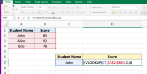
Since Formula requires four parameters, here First parameter is C7, in which we write John. Second parameter looks for Table, all the data contains, here, data is in A2 to B4, specified as absolute range($A$2:$B$4). Third parameter is column index which is 2 as we require detail of second column. Forth parameter is zero which means False, an exact match is required.
The result would be 85, which is John’s score.
VLOOKUP – Excel has this powerful formula , by combining with other functions and formulas to perform more complex tasks. Everyone, widely use it in various industries and professions to analyse and manipulate data in Excel.